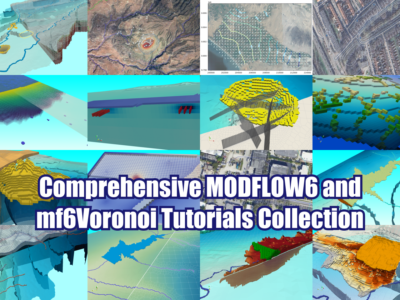
Simple example of construction site drainage modeling with MODFLOW6 and mf6Voronoi - Tutorial
/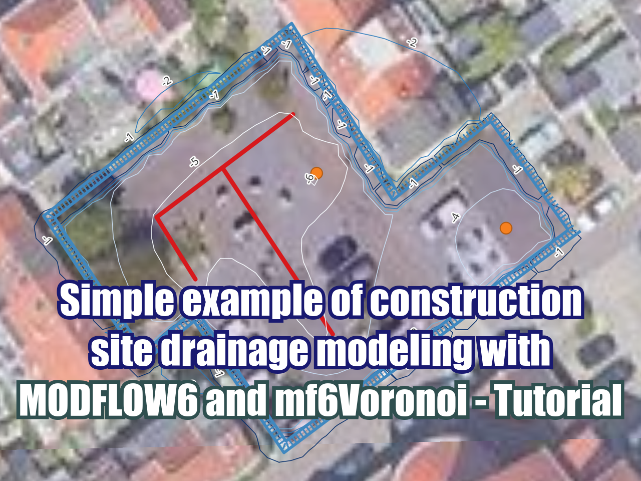
In mf6Voronoi horizontal flow barriers can be modeled as low k cells with thickness of 1m without compromising the cell amount and model performance. We have developed an applied case of construction site dewatering using horizontal drains and pumping wells that work in parallel over a period of 8 days. The model shows the performance of the drainage schema and exports the final water table as raster and contours.
Tutorial
Code
from mf6Voronoi.utils import listTemplates, copyTemplate#listTemplates()copyTemplate('generateVoronoi','wkExc')copyTemplate('multilayeredTransient','wkExc')Part 1 : Voronoi mesh generation
import warnings ## Org
warnings.filterwarnings('ignore') ## Org

import os, sys ## Org
import geopandas as gpd ## Org
from mf6Voronoi.geoVoronoi import createVoronoi ## Org
from mf6Voronoi.meshProperties import meshShape ## Org
from mf6Voronoi.utils import initiateOutputFolder, getVoronoiAsShp ## Org
#Create mesh object specifying the coarse mesh and the multiplier
vorMesh = createVoronoi(meshName='siteDewatering',maxRef = 10, multiplier=1) ## Org
#Open limit layers and refinement definition layers
vorMesh.addLimit('modelLimit','../shp/modelLimit.shp') ## Org
vorMesh.addLayer('hfb','../shp/hfb.shp',1) ## Org
vorMesh.addLayer('wells','../shp/pointWell.shp',1) ## Org
vorMesh.addLayer('drain','../shp/drains.shp',1) ## Org
vorMesh.addLayer('ghb','../shp/modelGhb.shp',3) ## Org#Generate point pair array
vorMesh.generateOrgDistVertices() ## Org
#Generate the point cloud and voronoi
vorMesh.createPointCloud() ## Org
vorMesh.generateVoronoi() ## Org
build faster, analyze more
Follow us: |
 |
 |
 |
 |
 |
 |
/--------Layer hfb discretization-------/
Progressive cell size list: [1, 2, 3, 4, 5, 6, 7, 8, 9, 10] m.

/--------Layer wells discretization-------/
Progressive cell size list: [1, 2, 3, 4, 5, 6, 7, 8, 9, 10] m.

/--------Layer drain discretization-------/
Progressive cell size list: [1, 2, 3, 4, 5, 6, 7, 8, 9, 10] m.

/--------Layer ghb discretization-------/
Progressive cell size list: [3, 6, 9] m.

/----Sumary of points for voronoi meshing----/
Distributed points from layers: 4
Points from layer buffers: 2440
Points from max refinement areas: 345
Points from min refinement areas: 0
Total points inside the limit: 2996
/--------------------------------------------/

Time required for point generation: 0.14 seconds


/----Generation of the voronoi mesh----/

Time required for voronoi generation: 0.14 seconds
#Uncomment the next two cells if you have strong differences on discretization or you have encounter an FORTRAN error while running MODFLOW6vorMesh.checkVoronoiQuality(threshold=0.005)/----Performing quality verification of voronoi mesh----/
Short side on polygon: 2995 with length = 0.00000
Short side on polygon: 2995 with length = 0.00000
Short side on polygon: 2995 with length = 0.00000
Short side on polygon: 2995 with length = 0.00000
Short side on polygon: 2995 with length = 0.00000
Short side on polygon: 2995 with length = 0.00000
Short side on polygon: 2995 with length = 0.00000
Short side on polygon: 2995 with length = 0.00000
Short side on polygon: 2995 with length = 0.00000
Short side on polygon: 2995 with length = 0.00000
Short side on polygon: 2995 with length = 0.00000
Short side on polygon: 2995 with length = 0.00000vorMesh.fixVoronoiShortSides()
vorMesh.generateVoronoi()
vorMesh.checkVoronoiQuality(threshold=0.005)/----Generation of the voronoi mesh----/
Time required for voronoi generation: 0.13 seconds
/----Performing quality verification of voronoi mesh----/
Your mesh has no edges shorter than your threshold#Export generated voronoi mesh
initiateOutputFolder('../output') ## Org
getVoronoiAsShp(vorMesh.modelDis, shapePath='../output/'+vorMesh.modelDis['meshName']+'.shp') ## OrgThe output folder ../output exists and has been cleared
/----Generation of the voronoi shapefile----/
Time required for voronoi shapefile: 0.25 seconds# Show the resulting voronoi mesh
#open the mesh file
mesh=gpd.read_file('../output/'+vorMesh.modelDis['meshName']+'.shp') ## Org
#plot the mesh
mesh.plot(figsize=(35,25), fc='crimson', alpha=0.3, ec='teal') ## Org
Part 2 generate disv properties
# open the mesh file
mesh=meshShape('../output/'+vorMesh.modelDis['meshName']+'.shp') ## Org
# get the list of vertices and cell2d data
gridprops=mesh.get_gridprops_disv() ## OrgCreating a unique list of vertices [[x1,y1],[x2,y2],...]
100%|██████████| 3051/3051 [00:00<00:00, 61237.31it/s]
Extracting cell2d data and grid index
100%|██████████| 3051/3051 [00:00<00:00, 6848.24it/s]#create folder
initiateOutputFolder('../json') ## Org
#export disv
mesh.save_properties('../json/disvDict.json') ## OrgThe output folder ../json exists and has been clearedPart 2a: generate disv properties
import sys, json, os ## Org
import rasterio, flopy ## Org
import numpy as np ## Org
import matplotlib.pyplot as plt ## Org
import geopandas as gpd ## Org
from mf6Voronoi.meshProperties import meshShape ## Org
from shapely.geometry import MultiLineString ## Org
from mf6Voronoi.tools.cellWork import getLayCellElevTupleFromRaster, getLayCellElevTupleFromElev
# open the json file
with open('../json/disvDict.json') as file: ## Org
gridProps = json.load(file) ## Orgcell2d = gridProps['cell2d'] #cellid, cell centroid xy, vertex number and vertex id list
vertices = gridProps['vertices'] #vertex id and xy coordinates
ncpl = gridProps['ncpl'] #number of cells per layer
nvert = gridProps['nvert'] #number of verts
centroids=gridProps['centroids'] #cell centroids xyPart 2b: Model construction and simulation
#Extract dem values for each centroid of the voronois
src = rasterio.open('../rst/modelDem.tif')  ## Org
elevation=[x for x in src.sample(centroids)] ## Org
nlay = 9 ## Org
mtop=np.array([elev[0] for i,elev in enumerate(elevation)]) ## Org
zbot=np.zeros((nlay,ncpl)) ## Org
zbot[0,] = mtop - 2
zbot[1,] = mtop - 4
zbot[2,] = mtop - 6
zbot[3,] = mtop - 8
zbot[4,] = mtop - 10
zbot[5,] = mtop - 14
zbot[6,] = mtop - 18
zbot[7,] = mtop - 22
zbot[8,] = mtop - 51Create simulation and model
# create simulation
simName = 'mf6Sim' ## Org
modelName = 'mf6Model' ## Org
modelWs = '../modelFiles' ## Org
sim = flopy.mf6.MFSimulation(sim_name=modelName, version='mf6', ## Org
                             exe_name='../bin/mf6.exe', ## Org
                             sim_ws=modelWs) ## Org
# create tdis package
tdis_rc = [(1.0, 1, 1.0), (86400*8, 1, 1.0)] ## pumping for eight days
print(tdis_rc[:3]) ## Org
tdis = flopy.mf6.ModflowTdis(sim, pname='tdis', time_units='SECONDS', ## Org
perioddata=tdis_rc, ## Org
nper=2) ## Org[(1.0, 1, 1.0), (691200, 1, 1.0)]# create gwf model
gwf = flopy.mf6.ModflowGwf(sim, ## Org
modelname=modelName, ## Org
save_flows=True, ## Org
newtonoptions="NEWTON UNDER_RELAXATION") ## Org# create iterative model solution and register the gwf model with it
ims = flopy.mf6.ModflowIms(sim, ## Org
complexity='COMPLEX', ## Org
outer_maximum=150, ## Org
inner_maximum=50, ## Org
outer_dvclose=0.1, ## Org
inner_dvclose=0.0001, ## Org
backtracking_number=20, ## Org
linear_acceleration='BICGSTAB') ## Org
sim.register_ims_package(ims,[modelName]) ## Org# disv
disv = flopy.mf6.ModflowGwfdisv(gwf, nlay=nlay, ncpl=ncpl, ## Org
top=mtop, botm=zbot, ## Org
nvert=nvert, vertices=vertices, ## Org
cell2d=cell2d) ## Orgdisv.top.plot(figsize=(12,8), alpha=0.8) ## Org
crossSection = gpd.read_file('../shp/crossSection.shp') ## Org
sectionLine =list(crossSection.iloc[0].geometry.coords) ## Org

fig, ax = plt.subplots(figsize=(12,8)) ## Org
modelxsect = flopy.plot.PlotCrossSection(model=gwf, line={'Line': sectionLine}) ## Org
linecollection = modelxsect.plot_grid(lw=0.5) ## Org
ax.grid() ## Org
# initial conditions

ic = flopy.mf6.ModflowGwfic(gwf, strt=np.stack([mtop for i in range(nlay)])) ## Org
#headsInitial = np.load('npy/headCalibInitial.npy')
#ic = flopy.mf6.ModflowGwfic(gwf, strt=headsInitial)
Kx = np.ones((nlay,ncpl))*4E-4
icelltype = [1, 1, 1, 1, 1, 0, 0, 0, 0]
#low k for horizontal flow barrier
interIx = flopy.utils.gridintersect.GridIntersect(gwf.modelgrid) ## Org
layCellTupleList = getLayCellElevTupleFromElev(gwf,
interIx,
0,
'../shp/hfb.shp')
#for the first two layers
for lay in range(5):
for layCellTuple in layCellTupleList:
Kx[lay,layCellTuple[1]] = 1e-10
# node property flow
npf = flopy.mf6.ModflowGwfnpf(gwf, ## Org
save_specific_discharge=True, ## Org
icelltype=icelltype, ## Org
k=Kx) ## Org
#k33=np.array(Kx))You have inserted a fixed elevationcrossSection = gpd.read_file('../shp/crossSection.shp') ## Org
sectionLine =list(crossSection.iloc[0].geometry.coords) ## Org
fig, ax = plt.subplots(figsize=(12,8)) ## Org
modelxsect = flopy.plot.PlotCrossSection(model=gwf, line={'Line': sectionLine}) ## Org
linecollection = modelxsect.plot_grid(lw=0.5) ## Org
linecollection = modelxsect.plot_array(npf.k.array, alpha=0.5) ## Org
ax.grid() ## Org
# define storage and transient stress periods
sto = flopy.mf6.ModflowGwfsto(gwf, ## Org
                              iconvert=1, ## Org
                              steady_state={ ## Org
                                0:True, ## Org
                              },
                              transient={
                                  1:True, ## Org
                              },
                              ss=1e-06,
                              sy=0.001,
                              ) ## Org
Working with rechage, evapotranspiration
rchr = 0.2/365/86400 ## Org
rch = flopy.mf6.ModflowGwfrcha(gwf, recharge=rchr) ## Org
evtr = 1.2/365/86400 ## Org
evt = flopy.mf6.ModflowGwfevta(gwf,ievt=1,surface=mtop,rate=evtr,depth=1.0) ## Org
Definition of the intersect object
For the manipulation of spatial data to determine hydraulic parameters or boundary conditions
# Define intersection object
interIx = flopy.utils.gridintersect.GridIntersect(gwf.modelgrid) ## Org
#ghb for regional flow
layCellTupleList = getLayCellElevTupleFromElev(gwf,
interIx,
0,
'../shp/modelGhb.shp')
ghbSpd = {} ## Org
ghbSpd[0] = [] ## Org
for index, layCellTuple in enumerate(layCellTupleList): ## Org
ghbSpd[0].append([layCellTuple,0,0.01]) ## Org
ghb = flopy.mf6.ModflowGwfghb(gwf, stress_period_data=ghbSpd) ## OrgYou have inserted a fixed elevation#ghb plot
ghb.plot(mflay=0, kper=0) ## Org
#drain package located at -6.0
layCellTupleList = getLayCellElevTupleFromElev(gwf,
                                               interIx,
                                               -6,
                                               '../shp/drains.shp')
drnSpd = {} ## Org
drnSpd[0] = [] ## Org
drnSpd[1] = []
for index, layCellTuple in enumerate(layCellTupleList): ## Org
    drnSpd[1].append([layCellTuple,-6,1]) ## Org

drn = flopy.mf6.ModflowGwfdrn(gwf, stress_period_data=drnSpd) ## Org
You have inserted a fixed elevation#drain plot
drn.plot(mflay=3, kper=1) ## Org
#well package located at -7.0
layCellTupleList = getLayCellElevTupleFromElev(gwf,
                                               interIx,
                                               -7,
                                               '../shp/pointWell.shp')
welSpd = {} ## Org
welSpd[0] = [] ## Org
welSpd[1] = []
for index, layCellTuple in enumerate(layCellTupleList): ## Org
    welSpd[1].append([layCellTuple,-0.015]) ## Org

wel = flopy.mf6.ModflowGwfwel(gwf, stress_period_data=welSpd) ## Org
You have inserted a fixed elevation#drain plot
wel.plot(mflay=4, kper=1) ## Org
Set the Output Control and run simulation
#oc
head_filerecord = f"{gwf.name}.hds" ## Org
budget_filerecord = f"{gwf.name}.cbc" ## Org
oc = flopy.mf6.ModflowGwfoc(gwf, ## Org
                            head_filerecord=head_filerecord, ## Org
                            budget_filerecord = budget_filerecord, ## Org
                            saverecord=[("HEAD", "LAST"),("BUDGET","LAST")]) ## Org
# Run the simulation
sim.write_simulation() ## Org
success, buff = sim.run_simulation() ## Orgwriting simulation...
writing simulation name file...
writing simulation tdis package...
writing solution package ims_-1...
writing model mf6Model...
writing model name file...
writing package disv...
writing package ic...
writing package npf...
writing package sto...
writing package rcha_0...
writing package evta_0...
writing package ghb_0...
INFORMATION: maxbound in ('gwf6', 'ghb', 'dimensions') changed to 151 based on size of stress_period_data
writing package drn_0...
INFORMATION: maxbound in ('gwf6', 'drn', 'dimensions') changed to 56 based on size of stress_period_data
writing package wel_0...
INFORMATION: maxbound in ('gwf6', 'wel', 'dimensions') changed to 2 based on size of stress_period_data
writing package oc...
FloPy is using the following executable to run the model: ..\bin\mf6.exe
MODFLOW 6
U.S. GEOLOGICAL SURVEY MODULAR HYDROLOGIC MODEL
VERSION 6.6.0 12/20/2024
MODFLOW 6 compiled Dec 31 2024 17:10:16 with Intel(R) Fortran Intel(R) 64
Compiler Classic for applications running on Intel(R) 64, Version 2021.7.0
Build 20220726_000000
This software has been approved for release by the U.S. Geological
Survey (USGS). Although the software has been subjected to rigorous
review, the USGS reserves the right to update the software as needed
pursuant to further analysis and review. No warranty, expressed or
implied, is made by the USGS or the U.S. Government as to the
functionality of the software and related material nor shall the
fact of release constitute any such warranty. Furthermore, the
software is released on condition that neither the USGS nor the U.S.
Government shall be held liable for any damages resulting from its
authorized or unauthorized use. Also refer to the USGS Water
Resources Software User Rights Notice for complete use, copyright,
and distribution information.
MODFLOW runs in SEQUENTIAL mode
Run start date and time (yyyy/mm/dd hh:mm:ss): 2025/10/28 11:07:33
Writing simulation list file: mfsim.lst
Using Simulation name file: mfsim.nam
Solving: Stress period: 1 Time step: 1
Solving: Stress period: 2 Time step: 1
Run end date and time (yyyy/mm/dd hh:mm:ss): 2025/10/28 11:07:38
Elapsed run time: 4.681 Seconds
Normal termination of simulation.Model output visualization
headObj = gwf.output.head() ## Org
headObj.get_kstpkper() ## Org
[(np.int32(0), np.int32(0)), (np.int32(0), np.int32(1))]kper = 1 ## Org
lay = 0 ## Orgheads = headObj.get_data(kstpkper=(0,kper))
#heads[lay,0,:5]
#heads = headObj.get_data(kstpkper=(0,0))
#np.save('npy/headCalibInitial', heads)### Plot the heads for a defined layer and boundary conditions
fig = plt.figure(figsize=(12,8)) ## Org
ax = fig.add_subplot(1, 1, 1, aspect='equal') ## Org
modelmap = flopy.plot.PlotMapView(model=gwf) ## Org
####
levels = np.linspace(heads[heads>-1e+30].min(),heads[heads>-1e+30].max(),num=50) ## Org
contour = modelmap.contour_array(heads[lay],ax=ax,levels=levels,cmap='PuBu')
ax.clabel(contour) ## Org
quadmesh = modelmap.plot_bc('DRN') ## Org
cellhead = modelmap.plot_array(heads[lay],ax=ax, cmap='Blues', alpha=0.8)
linecollection = modelmap.plot_grid(linewidth=0.3, alpha=0.5, color='cyan', ax=ax) ## Org
plt.colorbar(cellhead, shrink=0.75) ## Org
plt.show() ## Org
crossSection = gpd.read_file('../shp/crossSection.shp')
sectionLine =list(crossSection.iloc[0].geometry.coords)

waterTable = flopy.utils.postprocessing.get_water_table(heads)

fig, ax = plt.subplots(figsize=(12,8))
xsect = flopy.plot.PlotCrossSection(model=gwf, line={'Line': sectionLine})
lc = modelxsect.plot_grid(lw=0.5)
xsect.plot_array(heads, alpha=0.5)
xsect.plot_surface(waterTable)
xsect.plot_bc('wel', kper=kper, facecolor='none', edgecolor='crimson')
xsect.plot_bc('drn', kper=kper, facecolor='none', edgecolor='gold')
xsect.plot_grid(alpha=0.2)
plt.show()
from mf6Voronoi.tools.graphs2d import generateRasterFromArray, generateContoursFromRaster

wtPath = '../output/waterTable.tif'
generateRasterFromArray(gwf, waterTable,
                        rasterRes=1, epsg=32631,
                        outputPath=wtPath,
                        limitLayer='../shp/modelLimit.shp')
Raster X Dim: 301.76, Raster Y Dim: 290.48
Number of cols: 302, Number of rows: 291generateContoursFromRaster(wtPath, 1, '../output/wtContour.shp')
Input data
You can download the input data from this link:
owncloud.hatarilabs.com/s/zj1wW16jaKeamXM
Password: Hatarilabs